Why to avoid mean imputation (and try multiple imputation instead)
Anyone who has worked with data has discovered a fun secret: it has the tendency to have bits and pieces missing. That is, an observation may have values for some variables but not for others. A common strategy to deal with missing data is to replace missing values within a variable with the mean. Indeed, mean-imputation is one of the most commond methods for dealing with missing values. On the surface, its easy to see why this is an attractive approach. The original size of the dataset is maintained and the mean of the the variable remains unchanged. However, mean imputation comes with some drawbacks which we’ll explore below using the classic iris dataset. As an alternative, we’ll explore how multiple imputation can be used in place of mean-imputation focusing in on how estimates across imputed datasets are actually pooled.
##   Sepal.Length Sepal.Width Petal.Length Petal.Width Species
## 1          5.1         3.5          1.4         0.2  setosa
## 2          4.9         3.0          1.4         0.2  setosa
## 3          4.7         3.2          1.3         0.2  setosa
## 4          4.6         3.1          1.5         0.2  setosa
## 5          5.0         3.6          1.4         0.2  setosa
## 6          5.4         3.9          1.7         0.4  setosa

##              Sepal.Length Sepal.Width Petal.Length Petal.Width
## Sepal.Length    1.0000000  -0.1175698    0.8717538   0.8179411
## Sepal.Width    -0.1175698   1.0000000   -0.4284401  -0.3661259
## Petal.Length    0.8717538  -0.4284401    1.0000000   0.9628654
## Petal.Width     0.8179411  -0.3661259    0.9628654   1.0000000
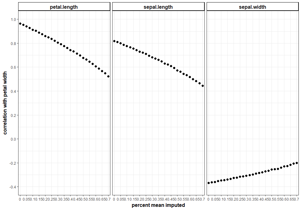
Replacing missing values with the mean distorts the relationship among variables
Specifically, the strength of the relationship between the other variables and the mean-imputed variable will decrease. Below, we’ll take the variable “Petal Width” and progressively, randomly remove a percentage of values and observe how that changes it’s relationship to other variables in the iris dataset. We’ll do this 500 times at each proportion of missingness and average the correlation between “Petal Width” and the 3 other numerical variables in the iris dataset. In this case, mean-imputing even a moderate about of data can have a pretty drastic effect on the relationship stucture of this dataset.

So, if we mean-impute, we distort the relationship structure of the data. What else can go wrong?
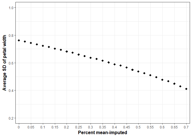
Mean-imputation leads to reduced variance
Intuitively this makes sense, you are plopping in the same value multiple times. Inherently, variability will be reduced. Once more, we’ll take the variable “Petal Width” and progressively, randomly remove a percentage of values and see how variance (SD) is affected. We’ll do this 500 times at each proportion of missingness and average the standard deviation of “Petal Width” at each step.

If the variance is reduced so is the standard error.
Statistics (e.g., one sample t-test) using the standard error to compute t-values and p-values will be biased potentially resulting in increased Type 1 error rates. Of course, this is far from ideal.
Solution?
Give multiple imputation a try.
A mean-based imputation is a single imputation strategy. With multiple imputation, several imputed datasets are created to account for the uncertainty in the imputation process. There are many algorithms that can be used to create these imputed datasets. A common number of imputed datasets to create is 5 or 10. Once these datasets are created, they are analyzed separately and their results pooled to arrive at a final result.
Pooling can be a confusing concept upon first exposure to multiple imputation methods. What (and how) exactly is being pooled? Let’s take a look.
The package “mice” is a popular package in R for performing multiple imputation. We’ll use it to impute some missing data from the variable “Petal Width”. In the “mice” function “m” is equal to the number of datasets we’ll be creating (here, m=5 which is the default). To impute, we’ll using predictive mean matching which is the default method.
library(mice)

miss <- prodNA(data.frame(iris$Petal.Width), noNA = .25)

temp.iris<-data.frame(iris[,1:3],miss)

imp.ris <- mice(temp.iris, m = 5,printFlag = FALSE)
When looking at the output we can see a few things. As stated above, the number of multiple imputations is equal to 5 and Predictive mean matching (pmm) was used as the imputation method. When looking at the “PredictorMatrix”, we can see that all the other variables in the iris dataset were used to create predicted values for “Petal Width”.
imp.ris
## Multiply imputed data set
## Call:
## mice(data = temp.iris, m = 5, printFlag = FALSE)
## Number of multiple imputations:  5
## Missing cells per column:
##     Sepal.Length      Sepal.Width     Petal.Length iris.Petal.Width
##                0                0                0               37
## Imputation methods:
##     Sepal.Length      Sepal.Width     Petal.Length iris.Petal.Width
##               ""               ""               ""            "pmm"
## VisitSequence:
## iris.Petal.Width
##                4
## PredictorMatrix:
##                  Sepal.Length Sepal.Width Petal.Length iris.Petal.Width
## Sepal.Length                0           0            0                0
## Sepal.Width                 0           0            0                0
## Petal.Length                0           0            0                0
## iris.Petal.Width            1           1            1                0
## Random generator seed value:  NA
As an example, let’s fit a simple regression model by regressing “Sepal Width” on “Petal Width”. Notice how a regression model is fit to each imputed dataset.
fit <- with(imp.ris, lm(iris.Petal.Width ~ Sepal.Width))
summary(fit)
##
##  ## summary of imputation 1 :
##
## Call:
## lm(formula = iris.Petal.Width ~ Sepal.Width)
##
## Residuals:
##     Min      1Q  Median      3Q     Max
## -1.4558 -0.5924 -0.0195  0.5191  1.6712
##
## Coefficients:
##             Estimate Std. Error t value Pr(>|t|)
## (Intercept)   3.1188     0.3995   7.807 9.85e-13 ***
## Sepal.Width  -0.6361     0.1294  -4.917 2.31e-06 ***
## ---
## Signif. codes:  0 '***' 0.001 '**' 0.01 '*' 0.05 '.' 0.1 ' ' 1
##
## Residual standard error: 0.6883 on 148 degrees of freedom
## Multiple R-squared:  0.1404, Adjusted R-squared:  0.1346
## F-statistic: 24.18 on 1 and 148 DF,  p-value: 2.308e-06
##
##
##  ## summary of imputation 2 :
##
## Call:
## lm(formula = iris.Petal.Width ~ Sepal.Width)
##
## Residuals:
##      Min       1Q   Median       3Q      Max
## -1.46164 -0.58897 -0.03628  0.52470  1.67541
##
## Coefficients:
##             Estimate Std. Error t value Pr(>|t|)
## (Intercept)   3.1426     0.4089   7.684 1.95e-12 ***
## Sepal.Width  -0.6439     0.1324  -4.862 2.94e-06 ***
## ---
## Signif. codes:  0 '***' 0.001 '**' 0.01 '*' 0.05 '.' 0.1 ' ' 1
##
## Residual standard error: 0.7046 on 148 degrees of freedom
## Multiple R-squared:  0.1377, Adjusted R-squared:  0.1319
## F-statistic: 23.64 on 1 and 148 DF,  p-value: 2.935e-06
##
##
##  ## summary of imputation 3 :
##
## Call:
## lm(formula = iris.Petal.Width ~ Sepal.Width)
##
## Residuals:
##      Min       1Q   Median       3Q      Max
## -1.54853 -0.58223 -0.01657  0.52109  1.66602
##
## Coefficients:
##             Estimate Std. Error t value Pr(>|t|)
## (Intercept)   3.0896     0.4062   7.606 3.03e-12 ***
## Sepal.Width  -0.6266     0.1315  -4.763 4.50e-06 ***
## ---
## Signif. codes:  0 '***' 0.001 '**' 0.01 '*' 0.05 '.' 0.1 ' ' 1
##
## Residual standard error: 0.6999 on 148 degrees of freedom
## Multiple R-squared:  0.1329, Adjusted R-squared:  0.1271
## F-statistic: 22.69 on 1 and 148 DF,  p-value: 4.503e-06
##
##
##  ## summary of imputation 4 :
##
## Call:
## lm(formula = iris.Petal.Width ~ Sepal.Width)
##
## Residuals:
##      Min       1Q   Median       3Q      Max
## -1.44252 -0.56779 -0.01756  0.53236  1.66973
##
## Coefficients:
##             Estimate Std. Error t value Pr(>|t|)
## (Intercept)   3.0796     0.4024   7.654 2.32e-12 ***
## Sepal.Width  -0.6248     0.1303  -4.795 3.92e-06 ***
## ---
## Signif. codes:  0 '***' 0.001 '**' 0.01 '*' 0.05 '.' 0.1 ' ' 1
##
## Residual standard error: 0.6933 on 148 degrees of freedom
## Multiple R-squared:  0.1345, Adjusted R-squared:  0.1286
## F-statistic: 22.99 on 1 and 148 DF,  p-value: 3.924e-06
##
##
##  ## summary of imputation 5 :
##
## Call:
## lm(formula = iris.Petal.Width ~ Sepal.Width)
##
## Residuals:
##      Min       1Q   Median       3Q      Max
## -1.43968 -0.57798 -0.03179  0.50663  1.66083
##
## Coefficients:
##             Estimate Std. Error t value Pr(>|t|)
## (Intercept)   3.0560     0.4072   7.505  5.3e-12 ***
## Sepal.Width  -0.6158     0.1319  -4.670  6.7e-06 ***
## ---
## Signif. codes:  0 '***' 0.001 '**' 0.01 '*' 0.05 '.' 0.1 ' ' 1
##
## Residual standard error: 0.7015 on 148 degrees of freedom
## Multiple R-squared:  0.1284, Adjusted R-squared:  0.1225
## F-statistic: 21.81 on 1 and 148 DF,  p-value: 6.703e-06
Now, estimates from the five regression models are pooled into 1 final result. But how?
summary(pool(fit))
##                    est        se         t       df     Pr(>|t|)
## (Intercept)  3.0973100 0.4065569  7.618393 144.4583 3.097966e-12
## Sepal.Width -0.6294298 0.1316414 -4.781395 144.5065 4.243603e-06
##                  lo 95      hi 95 nmis        fmi      lambda
## (Intercept)  2.2937414  3.9008785   NA 0.02178850 0.008338440
## Sepal.Width -0.8896212 -0.3692383    0 0.02157884 0.008130352
A common way to pool estimates involves combining the within and between imputation variability. To do this we need to grab the beta estimates and associated variances for each model.
b<-double()
v<-double()
for(i in 1:5){
b[i]<-fit$analyses[[i]]$coefficients[2]
v[i]<-vcov(fit$analyses[[i]])[2,2]
}

cbind(b,v)
##               b          v
## [1,] -0.6361127 0.01673606
## [2,] -0.6438847 0.01753770
## [3,] -0.6265744 0.01730438
## [4,] -0.6248033 0.01697810
## [5,] -0.6157738 0.01738663
Within variance is the average of the variances associated with beta estimates and between variance is a the variability in the beta estimates. The within and between variance are added to the between variance divded by a correction factor equal to the number of imputations (m). We can take the square root of this result to get the pooled standard error.
within_v<-mean(v)
between_v<-var(b)

sqrt(within_v+between_v+(between_v/5))
## [1] 0.1316414
Is multiple imputation worth the fuss?
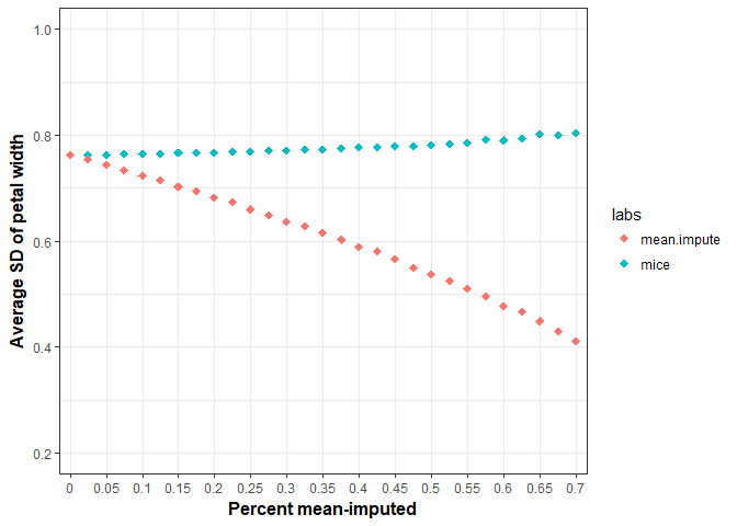
Yep. Let’s say we are botanists and wanted to test whether the mean petal width was different than some known value in the field. To do this theoretical one sample t-test we’d need to again pool variances across the imputed datasets. We can do this easily with the function “mi.t.test” from the “MKmisc” package. As before, we’ll take the variable “Petal Width” and progressively, randomly remove a percentage of values and see how variance (SD) is affected. We’ll perform multiple imputation with predicitive mean matching (m = 5) 500 times at each proportion of missingness and average the standard deviation of “Petal Width” at each step. These results are displayed along with the mean-imputation results from earlier. Note how stable SDs are in the multiply imputed data.

Hopefully, you’ll think twice about before mean-imputing and give multiple-imputaiton a shot.
There are of course other ways to handle missing data (e.g., KNN, random forest, etc) and there is no universal gold-standard when it comes to imputation. However, as I’ve shown, there are some methods (mean-imputation!) you’d do well to stay away from! Before thinking about imputing (or moving forward with the complete cases), its important to consider the structure of missing data whether it be missing completely at random (MCAR), missing at random (MAR), or missing not at random (MNAR) as this should impact your decision to impute (or not).