My first experience with regression and matrix algebra
As an undergraduate, regression was a fuzzy concept for me. I completed a year’s worth of psychology statistics, but in psychology ANOVA is king, and regression is alotted a whopping five pages in a chapter shared with correlation. After a sparse explanation of bivariate regression, multiple regression is usually mentioned as an afterthought on one page, something like the following:
“In the real world, an outcome is rarely explained by only one predictor. In this case, we can turn to multiple regression. Want to know more? Too bad” chapter ends on that note
Thus, the computations surrounding a more complex regression equation were very much a black box to me. Encouraged by a regression loving adviser, I decided to take a class titled, “Regression for Social and Behavioral Research” in the Statistics department to find out more about regression. During the first day of class we went over the syllabus:
- Week 1: An overview and review of OLS regression (review = good, I wont get left in the dust)
- Week 2: Mathmatical Derivation of Least Squares in Scalar Form (Things really escalated quickly)
- centeral concepts: where do regression coefficients and intercept come from? (yeah, where in the world do these things come from? I’d like to know, this sounds okay)
- Week 3: The Mathmetical Derivation of Least Squares in Matrix Form (uh-oh)
- central concepts: matrix maninpulations, eigenvalues, eigenvectors, cholesky decomposition, identity matrix (eigen what? Cholesky who?)
As a psychology student who had a fear of math drove into him, I went into shock and tuned out for the rest of class and missed learning more new funny sound words like, “probit” and “logit”. After the first day, I was 9000 percent set on dropping the class, but to my dismay “walking for fitness” was already full, so I was stuck in a class where I would spend the first month or so doing matrix algebra. Little did I know, this class would be one of (if not the best) classes I completed as an undergraduate and spurred my interest in data analysis and statistics.
My goal with this tutorial is to simply share some of the things I learned along the way with folks who completed a typical social science statistics course but were left not quite satisfied with how regression was introduced. We’ll unpack what is happening under the hood when you hit ctrl+enter on a line of code containing the function “lm”. I’m assuming the reader has a working knowledge of the basic concepts surrounding regression, so I won’t go over those in detail. The point of this post isn’t to spell all this out in complete mathematical proofs but to provide a hands on applied example of the concepts.
Time to dive in!
Let’s start by attaching the package “mtcars”. We will use some data from here as our dataset. We can see mtcars is a dataset composed of various information about cars including measures such as: mpg (miles per gallon), hp (horsepower), cyl (cylinders) etc …
data("mtcars")
head(mtcars,5)
##                    mpg cyl disp  hp drat    wt  qsec vs am gear carb
## Mazda RX4         21.0   6  160 110 3.90 2.620 16.46  0  1    4    4
## Mazda RX4 Wag     21.0   6  160 110 3.90 2.875 17.02  0  1    4    4
## Datsun 710        22.8   4  108  93 3.85 2.320 18.61  1  1    4    1
## Hornet 4 Drive    21.4   6  258 110 3.08 3.215 19.44  1  0    3    1
## Hornet Sportabout 18.7   8  360 175 3.15 3.440 17.02  0  0    3    2
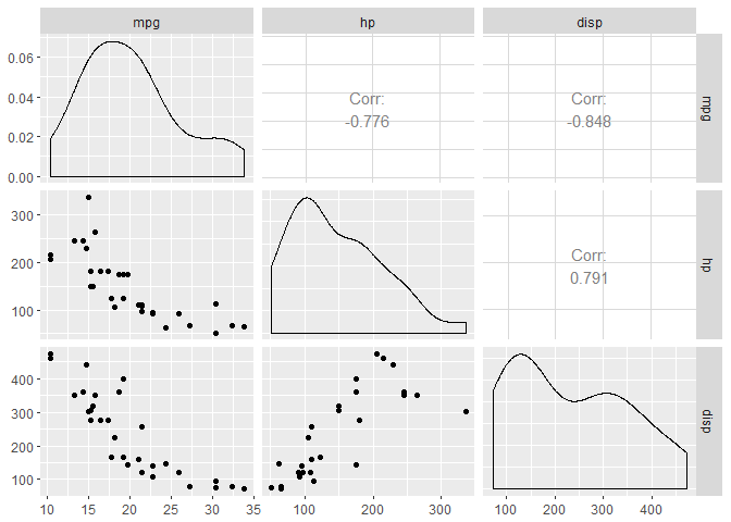
Let’s select 3 of these variables: mpg, hp, and disp (displacement). We’ll start by taking a quick peek at the data and by fitting a model with “lm” where we will be predicting mpg (y) from hp (x1) and disp (x2). We will then proceed to recreate the results of the lm summary from scratch.
library(ggplot2)
library(GGally)

ggpairs(mtcars[,c("mpg","hp","disp")])

summary(lm(mpg ~ hp + disp,data=mtcars))
##
## Call:
## lm(formula = mpg ~ hp + disp, data = mtcars)
##
## Residuals:
##     Min      1Q  Median      3Q     Max
## -4.7945 -2.3036 -0.8246  1.8582  6.9363
##
## Coefficients:
##              Estimate Std. Error t value Pr(>|t|)
## (Intercept) 30.735904   1.331566  23.083  < 2e-16 ***
## hp          -0.024840   0.013385  -1.856 0.073679 .
## disp        -0.030346   0.007405  -4.098 0.000306 ***
## ---
## Signif. codes:  0 '***' 0.001 '**' 0.01 '*' 0.05 '.' 0.1 ' ' 1
##
## Residual standard error: 3.127 on 29 degrees of freedom
## Multiple R-squared:  0.7482, Adjusted R-squared:  0.7309
## F-statistic: 43.09 on 2 and 29 DF,  p-value: 2.062e-09
Alright, now that we’ve seen the summary output, let’s get to work and re-create it! Our first step is to partition off our response and predictor variables into separate matrices.
y<-mtcars[,"mpg"]

x<-mtcars[,c("hp","disp")]
The next step is to finish our x matrix, or design matrix, which currently consists of our 2 predictor variables, hp and disp. To do this, we simply need to add a column (b0) representing the intercept. We can accomplish this by padding the current x matrix with a vector of ones.
x0<-rep(1,nrow(x))

x<-as.matrix(cbind(x0,x))

head(x,5)
##                   x0  hp disp
## Mazda RX4          1 110  160
## Mazda RX4 Wag      1 110  160
## Datsun 710         1  93  108
## Hornet 4 Drive     1 110  258
## Hornet Sportabout  1 175  360
Now, the fun begins
We’ll first start by finding our beta coefficients. In order to do this, we need to take the inverse of X transpose X and multiply that by X tranpose Y. Put more readably: \( b = (X^TX)^{-1}X^TY \). Below, we’ll begin by creating our \(X^TX \) and \(X^TY \) matrices.
XtX<-t(x)%*%x

XtY<-t(x)%*%y
Before calculating our regression coefficients, let’s pause for a second and check out this \(X^TX \) matrix. On the diagonal, you’ll find the sum squared values for our predictors and on the off-diagonal you’ll find the cross-products. To illustrate, we will calculate the sum of squares for hp and the cross product between hp and disp. You can see these values also appear in the appropriate spot in the \(X^TX \) matrix.
print(XtX)
##          x0      hp      disp
## x0     32.0    4694    7383.1
## hp   4694.0  834278 1291364.4
## disp 7383.1 1291364 2179627.5
sum(mtcars$hp*mtcars$hp)
## [1] 834278
sum(mtcars$hp*mtcars$disp)
## [1] 1291364
The \(X^TY \) matrix will take a bit of a different form as it will always be a vector of length n (number of covariates) + 1 (intercept), but you can still find the cross-products as seen below with respect to mpg and hp.
print(XtY)
##          [,1]
## x0      642.9
## hp    84362.7
## disp 128705.1
sum(mtcars$hp*mtcars$mpg)
## [1] 84362.7
Back to betas
Alright, time to calculate some regression coefficients. As mentioned earlier, \(b = (X^TX)^{-1}X^TY \). At this point, we have everything ready to plug into that formula, so we will go ahead and do so. Just to ensure that I’m not lying to you, we will compare out resulting calculation to that of lm.
betas<-solve(XtX)%*%XtY
betas
##             [,1]
## x0   30.73590425
## hp   -0.02484008
## disp -0.03034628
summary(lm(mpg ~ hp + disp,data=mtcars))$coefficients[1:3]
## [1] 30.73590425 -0.02484008 -0.03034628
Put a hat on it
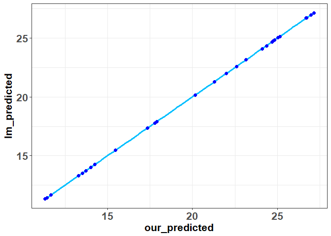
Now, we are going to compute something a little funky known as the hat matrix or projection matrix. This matrix is known as the hat matrix because it’s going to allow us map \(y \) into \(\hat{y} \). To find this hat matrix we need to use the following formula: \(H = X(X^TX)^{-1}X^T \). Once we have calculated the hat matrix, we multiple it by y to find our predicted values. We will do so, and compare our results to lm below:
hat_matrix<- x%*%solve(XtX)%*%t(x)

predicted<-hat_matrix%*%y

ggplot(data=data.frame(our_predicted=predicted,lm_predicted=lm(mpg ~ hp + disp,data=mtcars)$fitted.values),aes(x=our_predicted,y=lm_predicted))+geom_smooth(method=lm,se=FALSE,color="deepskyblue1",size=1.25)+geom_point(shape=19,color="blue",size=2)+theme_bw()+theme(axis.text=element_text(size=16,face="bold"),
        axis.title=element_text(size=16,face="bold"))

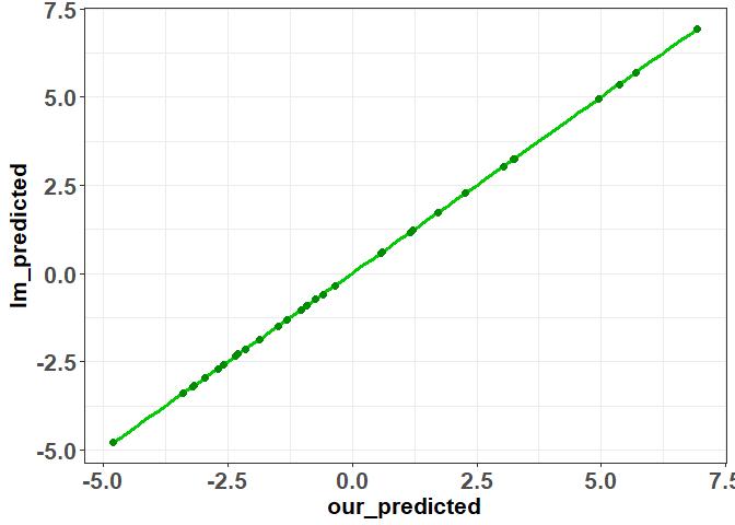
As you can see, everything matches up with the lm output. Now that we have our predicted values, we can easily find our residuals and again show that they are equal to the output produced by “lm”
residuals<-(y-predicted)

ggplot(data=data.frame(our_predicted=residuals,lm_predicted=lm(mpg ~ hp + disp,data=mtcars)$residuals),aes(x=our_predicted,y=lm_predicted))+geom_smooth(method=lm,se=FALSE,color="green3",size=1.25)+geom_point(shape=19,color="green4",size=2)+theme_bw()+theme(axis.text=element_text(size=16,face="bold"),
        axis.title=element_text(size=16,face="bold"))

An Estimate of Error
We can now use the residuals we’ve calculated to help us find the standard errors of our beta estimates. We can accomplish this by first finding the variance-covariance matrix between the regression coefficients. The formula to do so is: \(var(\hat{B}) = {\sigma^2}(X^TX)^{-1}\). To proceed we need to estimate \(\sigma^2\). To estimate \(\hat{\sigma^2}\) we can use the following formula \(\hat{\sigma^2} = \dfrac{1}{N-p}(r^Tr)\) where r is our vector of residuals, N = number of observations and p = number of columns in the design matrix (inctercept included). Once we have an estimate of variance, we can plug it in to the first formula to obtain our variance co-variance matrix. Once we have that, we can take the square root of its diaganol to obtain our standard errors. As usual, we will compare our calculations to “lm”.
var_est <- (1/(nrow(x)-ncol(x)))*t(residuals)%*%residuals
ses<-sqrt(diag(as.numeric(var_est)*solve(XtX)))
print(ses)
##          x0          hp        disp
## 1.331566129 0.013385499 0.007404856
summary(lm(mpg ~ hp + disp,data=mtcars))$coefficients[4:6]
## [1] 1.331566129 0.013385499 0.007404856
Finishing up
Now, we can complete our calculations by obtain t and p - values. We can even calculate a few other things lm gives you such as r2 and adjusted r2.
tvals<-betas/ses
print(tvals)
##           [,1]
## x0   23.082522
## hp   -1.855746
## disp -4.098159
pvals<-sapply(tvals, function (p) 2*pt(abs(-p), nrow(x)-ncol(x), lower=FALSE))
print(pvals)
## [1] 3.262507e-20 7.367905e-02 3.062678e-04
r2<-sum((predicted-mean(y))^2)/sum((y-mean(y))^2)
print(r2)
## [1] 0.7482402
adjusted_r2<-1-(((1-r2)*(nrow(x)-1))/(nrow(x)-(ncol(x)-1)-1))
print(adjusted_r2)
## [1] 0.7308774
Finally, we can combine everything in one spot and compare it to the summary output of lm.
round(data.frame(b=betas,se=ses,t_value = tvals,p_value=pvals,r2=c(r2,rep(NA,2)),adj_r2=c(adjusted_r2,rep(NA,2))),6)
##              b       se   t_value  p_value      r2   adj_r2
## x0   30.735904 1.331566 23.082522 0.000000 0.74824 0.730877
## hp   -0.024840 0.013385 -1.855746 0.073679      NA       NA
## disp -0.030346 0.007405 -4.098159 0.000306      NA       NA
summary(lm(mpg ~ hp+disp,data=mtcars))
##
## Call:
## lm(formula = mpg ~ hp + disp, data = mtcars)
##
## Residuals:
##     Min      1Q  Median      3Q     Max
## -4.7945 -2.3036 -0.8246  1.8582  6.9363
##
## Coefficients:
##              Estimate Std. Error t value Pr(>|t|)
## (Intercept) 30.735904   1.331566  23.083  < 2e-16 ***
## hp          -0.024840   0.013385  -1.856 0.073679 .
## disp        -0.030346   0.007405  -4.098 0.000306 ***
## ---
## Signif. codes:  0 '***' 0.001 '**' 0.01 '*' 0.05 '.' 0.1 ' ' 1
##
## Residual standard error: 3.127 on 29 degrees of freedom
## Multiple R-squared:  0.7482, Adjusted R-squared:  0.7309
## F-statistic: 43.09 on 2 and 29 DF,  p-value: 2.062e-09
Coming up next
Hopefully you now have a clearer understand of the computations behind a regression model! One thing to note, is that this post dealt with solely numeric predictor variables and no interaction terms. In the next post, we will extend our design matrix to include those cases as well. To keep things neat, we will also synthesize the code we wrote and create our own “lm” function that takes in a response vector and design matrix and outputs a regression summary.